Sensitivity analysis using FabSim3 and EasyVVUQ
FabSim3 is very useful when submitting a large number of jobs at together. One of the cases where this becomes especially useful is for sensitivity analysis. Sensitivity analysis can be breifly described as the process of evaluating the extent to which various input parameters affect the output of a simulation. One of the popular ways of quantifying this effect of parameters on the simulations is throgh Sobol Indices. Computation of Sobol Indices involves running the simulation for a large number of parameter sets and then comuting the variances among the various subsets of results obtained. Given the large number of computations required, this becomes a suitable candidate for simplification using FabSim3.
In this tutorial, we showcase how to conduct sensitivity analysis using FabSim3 and the python packages EasyVVUQ and QCG-PilotJob. The tutorial will use a simple plugin called FabDynamics which has been tailored for this purpose.
Brief introduction of Dynamics and FabDynamics
At the core of this tutorial is the Dynamics software which numerically solves a system of differential equations for a fixed amount of time. By default, if no arguments are provided, the program solves the FitzHugh-Nagumo system of differential equations:
where \(a\), \(b\) and \(c\) are three real-valued parameters that determine the time-evolution of dynamical variables \(x\) and \(y\).
In order to use FabSim3 with the Dynamics software, we use the FabDynamics plugin. This plugin would help us submit large ensembles of simulation runs and perform sensitivity analysis. We discuss this aspect of the plugin in the following sections of the tutorial.
Installing Dynamics
In order to install the Dynamics software:
-
Clone the software repository in a directory of your choice:
2. Enter the newly created directory:git clone https://github.com/arindamsaha1507/dynamics.gitcd dynamics -
Install the required dependencies:
pip install -r requirements.txt -
This should complete the installation process. Check that the software works properly by issuing the command:
This should create a new file calledpython run.pytimeseries.csvwhich contains the time-evolution of variables \(x\) and \(y\). -
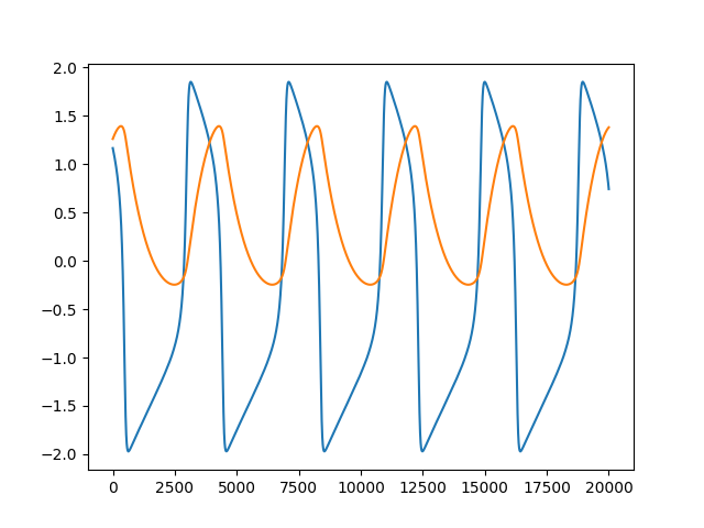
To check that the results are as expected, you can plot the results using:
This should result in a plot similar to the one shown below.python plotter.py
Installing FabDynamics
Now, with the Dynamics software installed, we must install the FabDynamics plugin so that we can use it with FabSim3:
-
With FabSim3 installed properly, issue the following command:
This should create afabsim localhost install_plugin:FabDynamicsFabDynamicssubdirectory in theFabSim3/pluginsdirectory. -
Change to the newly created directory:
cd <path to FabSim3 directory>/plugins/FabDynamics -
Copy the contents of the
machines_FabDynamics_user_example.ymlfile into a new filemachines_FabDynamics_user.yml:cp machines_FabDynamics_user.yml machines_FabDynamics_user_example.yml -
Now edit the the last line of the
machines_FabDynamics_user.ymlfile with the location where dynamics software is installed:default: dynamics_args: outfile: 'timeseries.csv' localhost: # location of dynamics in your local PC dynamics_location: "<path/to/dynamics/software>"
Perfoming sensitivity analysis and computing Sobol Indices
The FabDynamics plugin comes pre-configured for sensitivity analysis. In order to start sensitivity analysis with default settings, simply issue the command:
fabsim localhost dyn_init_SA:config=fhn
Note
If you wish to use QCG-PilotJob during the SA runs on HPC's, simply modify the command as
fabsim <machine_name> dyn_init_SA:config=fhn,PJ=True
Based on the pre-set configuration, issuing this command selects 64 points in the three-dimensional parameter space defined by parameters \(a\), \(b\) and \(c\). It then submits one simulation run for each parameter set to the localhost.
After all the simulation runs have successfully run, the results of the simulations can be collected and analysed using a single command:
fabsim localhost dyn_analyse_SA:config=fhn
Issuing this command also computes the Sobol indices at each point in the timeseries. The results of this analysis are stored in the directory:
<path to FabSim3 directory>/plugins/FabDynamics/SA/dyn_SA_SCSampler
In this directory
-
The first order Sobol indices are stored in
sobols.yml. The contents of this file should look like:campaign_info: name: "dyn_SA_SCSampler" work_dir: "/home/arindam/FabSim3/plugins/FabDynamics" num_runs: 64 output_column: "x" polynomial_order: 3 sampler: "SCSampler" distribution_type: "Uniform" sparse: "False" growth: "False" quadrature_rule: "G" midpoint_level1: "False" dimension_adaptive: "False" a: # arithmetic mean i.e., (x1 + x2 + … + xn)/n sobols_first_mean: 0.435 # geometric mean, i.e., n-th root of (x1 * x2 * … * xn) sobols_first_gmean: 0.4329 sobols_first: [0.5201, 0.5201, 0.5201, 0.5201, 0.52, 0.52, 0.52, 0.5199, 0.5199, 0.3959, 0.3956, 0.3953, 0.395, 0.3947, 0.3945, 0.3942, 0.3938, 0.3935] b: # arithmetic mean i.e., (x1 + x2 + … + xn)/n sobols_first_mean: 0.011 # geometric mean, i.e., n-th root of (x1 * x2 * … * xn) sobols_first_gmean: 0.0085 sobols_first: [0.0042, 0.0042, 0.0041, 0.0041, 0.004, 0.004, 0.004, 0.0039, 0.0039, 0.0039, 0.0038, 0.0038, 0.0037, 0.0037, 0.0037, 0.0036, 0.0036, 0.0036, 0.0036, 0.0035, ... 0.0069, 0.007, 0.007, 0.007, 0.0071, 0.0071, 0.0072, 0.0072, 0.0073, 0.0073] c: # arithmetic mean i.e., (x1 + x2 + … + xn)/n sobols_first_mean: 0.0382 # geometric mean, i.e., n-th root of (x1 * x2 * … * xn) sobols_first_gmean: 0.0288 sobols_first: [0.0097, 0.0098, 0.0099, 0.01, 0.0101, 0.0102, 0.0103, 0.0104, 0.0105, 0.0106, 0.0107, ... 0.0197, 0.0195, 0.0194, 0.0192, 0.0191, 0.0189, 0.0188, 0.0186, 0.0185, 0.0183, 0.0182]As evident from the contents of the file, the first order Sobol indices for each parameter is computed separately.
-
The plot of the first-order Sobol indices is stored in
plot_sobols_first[x].png. The plot should look similar to:

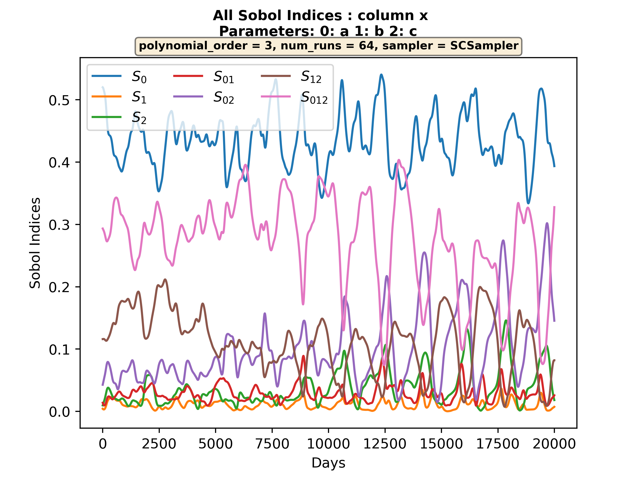
- Similar plot showing all Sobol indices (inclding the higher order indices) is stored in
plot_all_sobol[x].png. The plot should look similar to:
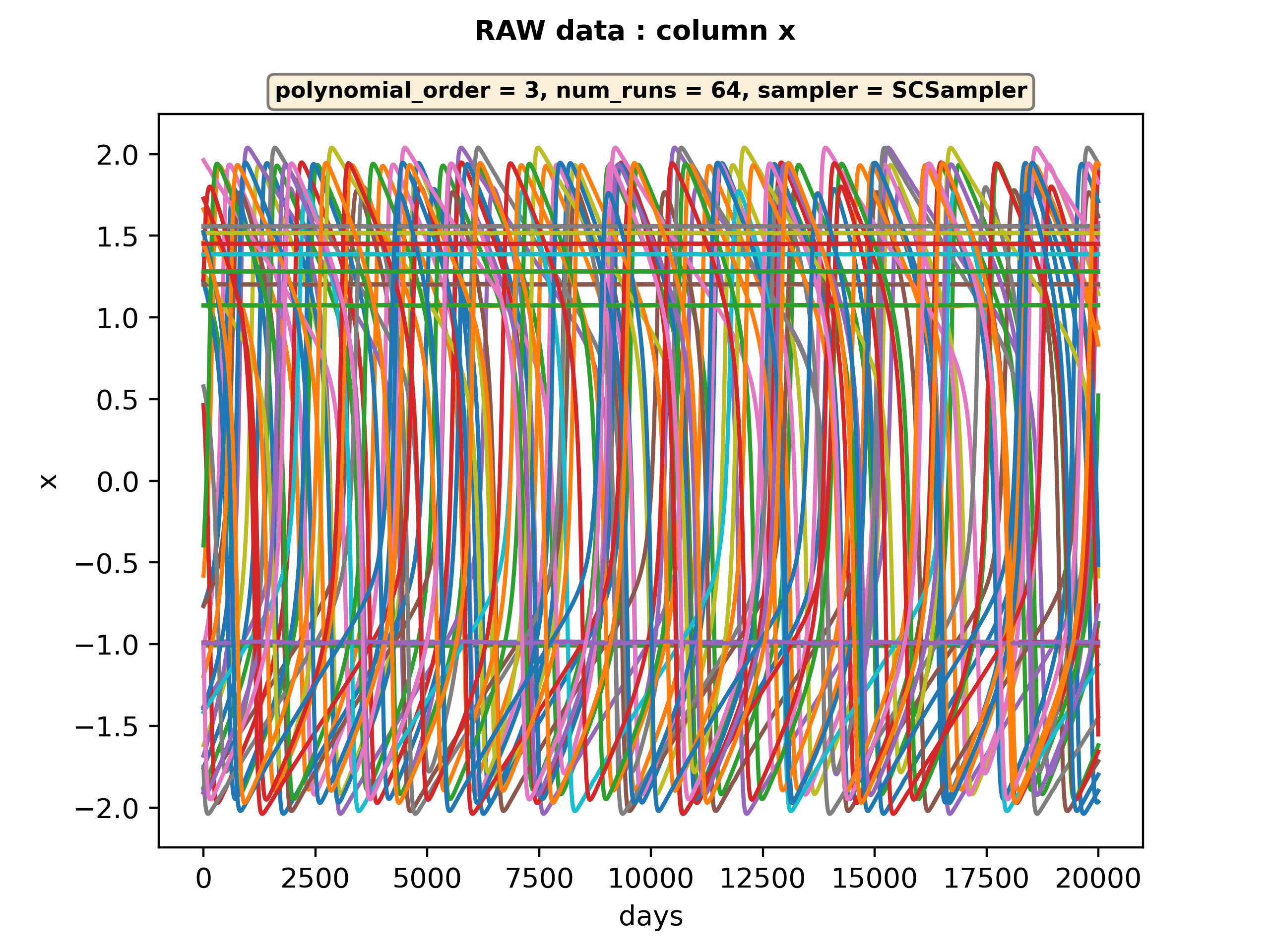
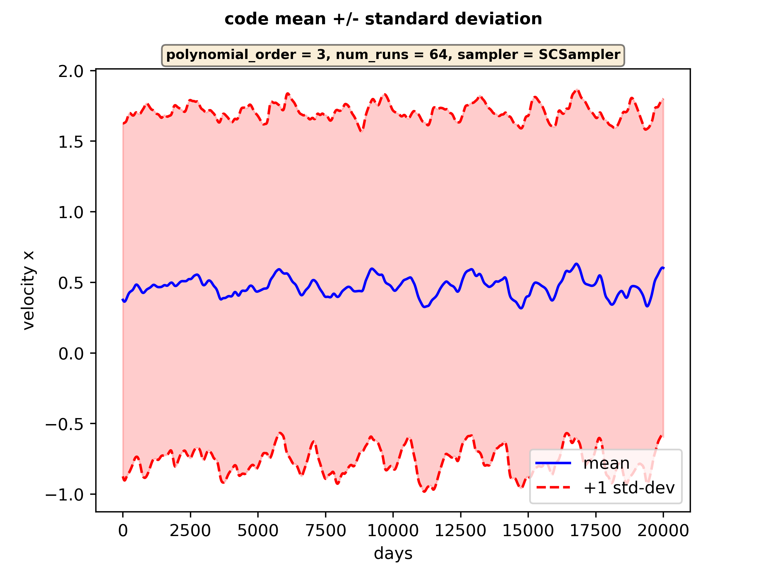
- The command also creates other plots related to the results of the simulation runs, namely
raw[x].pngandplot_statistical_moments[x].png.
Configuring sensitivity analysis
After the steps taken above, the dirctory structure of the FabDynamics plugin should look like:
FabDynamics
├── config_files
│   ├── fhn
│   └── testing
├── FabDynamics.py
├── LICENSE
├── machines_FabDynamics_user_example.yml
├── machines_FabDynamics_user.yml
├── __pycache__
│   ├── FabDynamics.cpython-310.pyc
│   └── FabDynamics.cpython-38.pyc
├── README.md
├── requirements.txt
├── SA
│   ├── dyn_SA_config.yml
│   ├── dyn_sa.py
│   ├── dyn_SA_SCSampler
│   └── __pycache__
└── templates
    ├── dynamics
    ├── params.json
    └── template_inputs
Out of these files, the following determine the configuration for senstivity analysis:
The dyn_sa.py module contains the central function that controls the sensitivity analysis. So, when we issue the command:
fabsim localhost dyn_init_SA:config=fhn
The following function in dyn_sa.py is run:
@task
@load_plugin_env_vars("FabDynamics")
def dyn_init_SA(config,
                outdir=".",
                script="dynamics",
                dynamics_script="run.py",
                sampler_name=None,
                ** args):
with the argument config=fhn.
After the required pre-processing, this function creates an EasyVVUQ campaign in the following line:
runs_dir, campaign_dir = init_dyn_SA_campaign(
        campaign_name=campaign_name,
        campaign_config=dyn_SA_campaign_config,
        polynomial_order=polynomial_order,
        campaign_work_dir=campaign_work_dir,
        template='template_inputs',
        target='inputs.yml'
    )
The specifics of how the sensitivity analysis campaign would work is defined in the arguments of the init_dyn_SA_campaign() function. In particular, the template='template_inputs' and target='inputs.yml' arguments specify that the inputs.yml configuration file for the individual run has to be formatted according to the template_inputs template file.
Let us have a look at the inputs.yml file in the FabDynamics/config_files/fhn/configuration/ directory:
family: 'ode'

ode_system: 'fhn'

parameters:
  a:
    min: -1.0
    max: 1.0
    default: 0.7
  b:
    min: 0.0
    max: 1.0
    default: 0.8
  c:
    min: 0.0
    max: 20.0
    default: 12.5

initial_conditions:
  x:
    min: -5.0
    max: 5.0
    default: 0.1
  y:
    min: -5.0
    max: 5.0
    default: 0.1

time:
  ti: 0.0
  tf: 1000.0
  dt: 0.01
  tr: 0.8
This is very similar to the template_inputs template file in the FabDynamics/templates/ directory:
family: 'ode'

ode_system: 'fhn'

parameters:
  a:
    min: -1.0
    max: 1.0
    default: $a
  b:
    min: 0.0
    max: 1.0
    default: $b
  c:
    min: 0.0
    max: 20.0
    default: $c

initial_conditions:
  x:
    min: -5.0
    max: 5.0
    default: 0.1
  y:
    min: -5.0
    max: 5.0
    default: 0.1

time:
  ti: 0.0
  tf: 1000.0
  dt: 0.01
  tr: 0.8
In fact, the only difference between the two files is that instaed of numerical values for keys a, b and c, the template file contains symbols $a, $b and $c.
Essentially the init_dyn_SA_campaign() function copies the template='template_inputs' into target='inputs.yml' file after substituting the $ variables with numerical values. The algorithm by which the numerical values are substituted are determined by dyn_SA_config.yml and params.json files.
Let us look at the dyn_SA_config.yml file:
vary_parameters_range:
    # <parameter_name:>
    #   range: [<lower value>,<upper value>]
    a:
        range: [-1.0, 1.0]
    b:
        range: [0.5, 0.9]
    c:
        range: [12.0, 13.0]

selected_vary_parameters: ["a",
                           "b",
                           "c",
                          ]

distribution_type: "Uniform" # Uniform, DiscreteUniform

polynomial_order: 3

decoder_output_column: "x"

#   ---------------------------------------------------------------
# sampler_name: str
#   Samplers in the context of EasyVVUQ are classes that generate
#   sequences of parameter dictionaries.
#   available sampler: [SCSampler,PCESampler]
#
#   SCSampler: Stochastic Collocation sampler
#   PCESampler : Polynomial Chaos Expansion
#   ---------------------------------------------------------------
sampler_name: "SCSampler"


# quadrature_rule : char
#     The quadrature method, default is Gaussian "G".
#     "G" -> Gaussian , "C" -> Clenshaw_Curtis
quadrature_rule: "G"

# ------- NOTE ------------
# if you set quadrature_rule="C", then you need to make sure
#     sparse=True
#     growth=True
#     midpoint_level1=True


# sparse : bool
#             If True use sparse grid instead of normal tensor product grid,
#             default is False
sparse: False

# growth: bool
#     Sets the growth rule to exponential for Clenshaw Curtis quadrature,
#     which makes it nested, and therefore more efficient for sparse grids.
#     Default is False.
growth: False

# midpoint_level1: bool,  ----- ONLY FOR SCSampler ------
#     determines how many points the 1st level of a sparse grid will have.
#     If midpoint_level1 = True, order 0 quadrature will be generated
midpoint_level1: False

# dimension_adaptive: bool, ----- ONLY FOR SCSampler ------
#     determines wether to use an insotropic sparse grid, or to adapt
#     the levels in the sparse grid based on a hierachical error measure
dimension_adaptive: False

# regression: bool, ----- ONLY FOR PCESampler ------
#    If True, regression variante (point collecation) will be used,
#    otherwise projection variante (pseud-spectral) will be used.
#    Default value is False.
regression: False
This file determines the overall configuration of the sensitivity analysis. In particular, the key selected_vary_parameters determines the variables with respect to which the sensitivity analysis is to be performed. Therefore, in the example, variables a, b abd c would be varied. The ranges in which the variables will be varied is determined by the vary_parameters_range key.
Therefore, during the analysis in the example, the parameters are scanned in a three-dimensional space. The granularity with which the parameter space is scanned is determined by the polynomial_order key. With a polynomial_order of \(n\), a total of \(n+1\) samples will be taken for each parameter. If there are a total of \(p\) parameters to be varied, there will be a total of \((n+1)^p\) samples taken from the parameter space. Therefore, in the example above an ensemble size of \(4^3=64\) will be created.
The decoder_output_column key in the dyn_SA_config.yml file determines the column in the output file based on which the the Sobol indices are to be computed. In addition, the file also determines other factors such as the sampler and other EasyVVUQ specific parameters. These are explained in detain in the comments of the file.
Finally, we note the role of params.json file in configuring the sensitivity analysis. Let us first look at the file:
{
    "a": {
      "type": "float",
      "min": -1.0,
      "max": 1.0,
      "default": 0.7
    },
    "b": {
      "type": "float",
      "min": 0.0,
      "max": 1.0,
      "default": 0.8
    },
    "c": {
      "type": "float",
      "min": 0.0,
      "max": 20.0,
      "default": 12.5
    },
    "out_file": {
      "type": "string",
      "default": "timeseries.csv"
    }
}
The file first lists the variables that are allowed to be varied, which are a, b and c. It also lists the out_file variable which gives the file in which the output file will be written.
Similar to the dyn_SA_config.yml file, the params.json file also states a mininum and a maximum value of the parameters. This is because, the params.json file is meant to be system-specific, whereas the dyn_SA_config.yml file is meant to be spficit to the current sensitivity analysis run. Hence, the limits set in params.json file are supposed to be the theoretical limits of the variables. However, the limits in the dyn_SA_config.yml file determines the actual limits within which the values of the variables will be varied during the sensitivity analysis. Therefore, the limits set in dyn_SA_config.yml must be a subset of the limits set in params.json file.
The params.json file also specifies a default value for each variable. This is the value given to the variable when it is not being used in a particular run of sensitivity analysis. Therefore, if the selected_vary_parameters key in the dyn_SA_config.yml file is set to [a, b], value of $c that will be substitute in template_inputs will be 12.5 as that is the default value assigned to c in params.json file.